The goal in this section is to generate a graph visualization (see the very bottom of this post) for each Pubski and in the process, extract and note various properties. Then we can measure how these properties change (or don't) over time, and see if we can learn something about online commnunities.

If you'd like to browse some of the code created/used in this section, it's available here: https://github.com/SeanCLynch/pubski_analysis.

This post is divided into three parts:
(1) anecdote and adventure from Pubski
(2) a network-based exploration of Pubski (this post), and
(3) some formal anthropological/sociological thoughts on Pubski.

Basic Data Gathering

Navigate to Hubski and search for #pubski. Scroll to the bottom and click "more" until there are no more posts to load. I then saved this page, so that I could politely query it without hitting the live servers. Now we have a pubski_list.html file!

Next, I loaded that page in my browser (right click, open with...), and iteratively experimented until I produced the following code snippet, which is run in the browser console. It outputs a JSON array of the posts with their relevant info, which you can right-click on (in the browser console) and save as pubski_list.json.

let pubs_divs = document.querySelectorAll('#unit');
let pubs_array = [];
pubs_divs.forEach(function (pub, idx) { 
  let hubwheel = pub.querySelector('.plusminus .score a').className;
  let hubwheel_dots = hubwheel.slice(-1);

  let title	= pub.querySelector('.feedtitle span a span').innerText;
  let post_date	= title.slice(7);
  let post_link	= pub.querySelector('.feedtitle span a').getAttribute('href');

  let comment_count = pub.querySelector('.feedcombub > a').innerText;
  let top_commenter = pub.querySelector('.feedcombub a').innerText;
        
  let badges = pub.querySelector('.titlelinks a.ajax');
  let multiple_badges = pub.querySelector('.titlelinks a.ajax b');
  let num_badges = 
    (multiple_badges ? 
        multiple_badges.innerText.slice(-1) : 
        badges ? 1 : 0);

  pubs_array.push({
    "title": title,
    "post_date": post_date,
    "post_link": post_link,
    "comment_count": comment_count,
    "top_commenter": top_commenter,
    "hubwheel_dots": hubwheel_dots,
    "num_badges": num_badges
  });
});

console.log(pubs_array);

Next, I wanted to convert the JSON into a CSV, so that I could use spreadsheet software to make pretty graphs. I hadn't used 'jq' before but had heard good things, so in the terminal I typed: sudo apt-get install jq. Then, after some searching around, I found some docs & some code snippets that led me to create the following code, which outputs a pubski_list.csv file. To be entirely frank, I'm not sure I fully grasp how jq in this snippet works, but I can't argue with the output!

cat pubski_list.json | jq -r '(.[0] | keys_unsorted) as $keys | $keys, map([.[ $keys[] ]])[] | @csv' > pubski_list.csv

I also manually combed through the data, checking for any anomlies and found two things. First, that there are exactly three posts that used the '#pubski' and were not related to the weekly post whatsoever. It's very likely that these users were posting about a topic, and the Hubski recommendation system suggested '#pubski'. These posts were deleted prior to data processing. Here are those posts:

• Realbeer.com: Beer News: The most beers on tap?, http://www.realbeer.com/news/articles/news-000246.php, 0 comments
• Pico countertop craft automatic brewery for the inexperienced home brewer, http://www.gizmag.com/pico-countertop-automated-craft-beer-brewing-machine/40063/, 0 comments
• Introducing Glyph, https://endlesswest.com/glyph/, 2 comments

The other anomly was two 'meta' posts about Pubski. Both related to the timing of Pubski and the belief that something was disrupting the normal scheduling of Pubski. These were kept in the dataset prior to processing. You can see them below:

• 'Pubski: July 25, 2018 [closed]', http://hubski.com/pub/412363, 10 comments
• 'Is it just me or was there no pubski last week?', http://hubski.com/pub/424500, 4 comments

Basic Data Processing

Using the data (pubski_list.json and pubski_list.csv), I could easily measure technical and social attributes of Pubski, like number of Pubski posts (total 300), comment count (average 77), badge count (average 1, median 0), most common top_commentor (kleinbl00, 28 times, in 11% of Pubski posts), first post id (172369). I can even create more advanced charts like these:

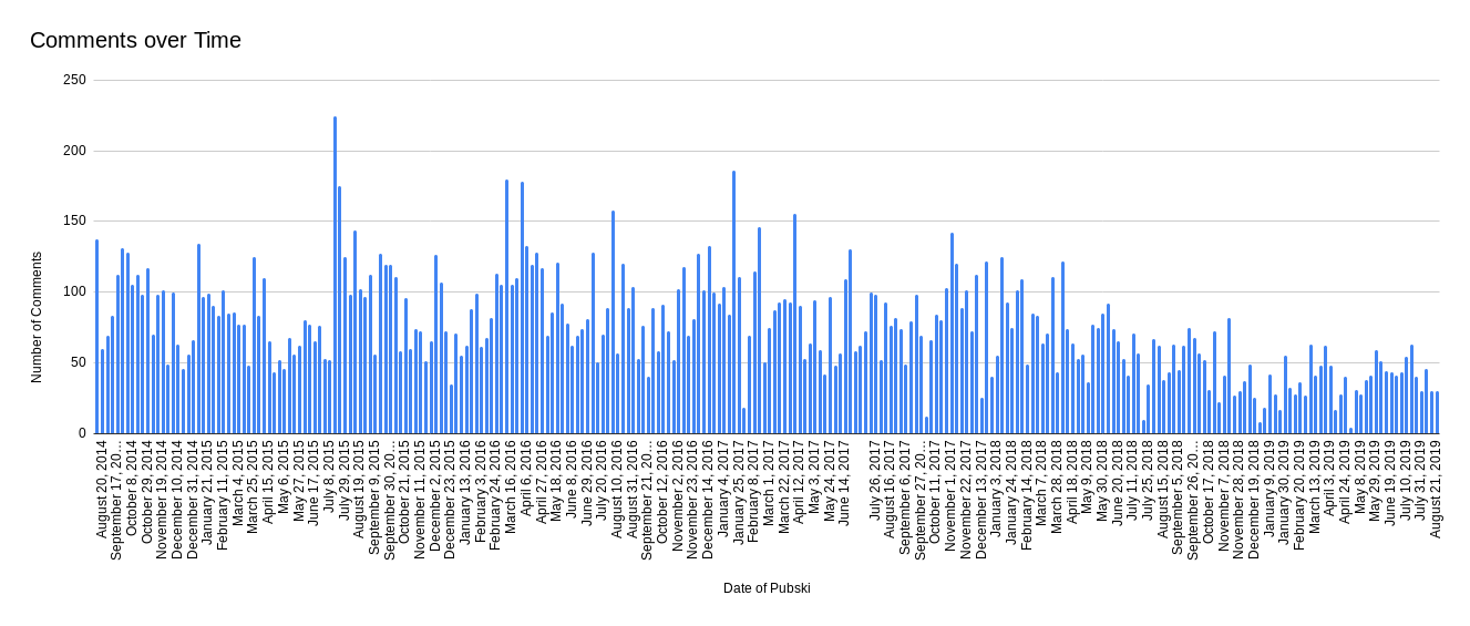
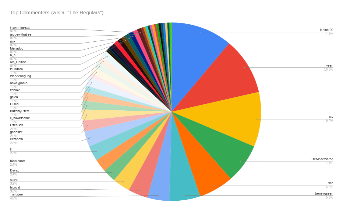
All of this data is nice, but doesn't tell us too much about any individual Pubski, so let's dig deeper!

Advanced Data Gathering

Now, with the list of (hundreds of) Pubski posts in JSON & CSV, I could start to think about how we might crawl the list of Pubski links and get static versions of each individual page. The technique I ended up using was a NodeJS script to fetch and parse each page into two formats: a list of nodes and edges (and metadata) in JSON and an edgelist text file. These are two data formats that effectively represent each Pubski in a graph or network format (where users are nodes, and edges represent one user replying to the other). The edgelist file could then be read by a Python script, wherein we could plot the graph visually and perform various algorithms on it.

The first script I called getAllPosts.js, you can see it on Github here.

The second script I called analyzePosts.py, you can see it on Github here.

Advanced Data Processing

Now, given the CSV produced by analyzePosts.py, I could get down to the business of looking for trends and patterns. Now, staring at numbers in a spreadsheet is mind-numbing, so I created plots of the data in Google Sheets. Below are 10 metrics with brief explainations before we dive into interpreting the data in the next seection.

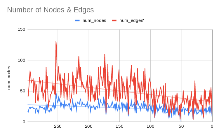
1. First is a pretty straightforward measure, the number of nodes and number of edges in each pubski. You can see that while the number of nodes (participants) is relatively stable, the number of edges (posts/replys) is on a slight downward trend.

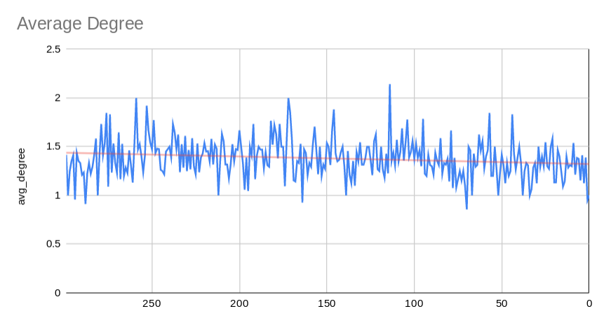
2. Second is the average degree. The degree of a given node is defined as the number of edges incident to it. So one node with two outgoing edges (replys) has a degree of 2. This measure seems to have remained fairly stable around 1.4.

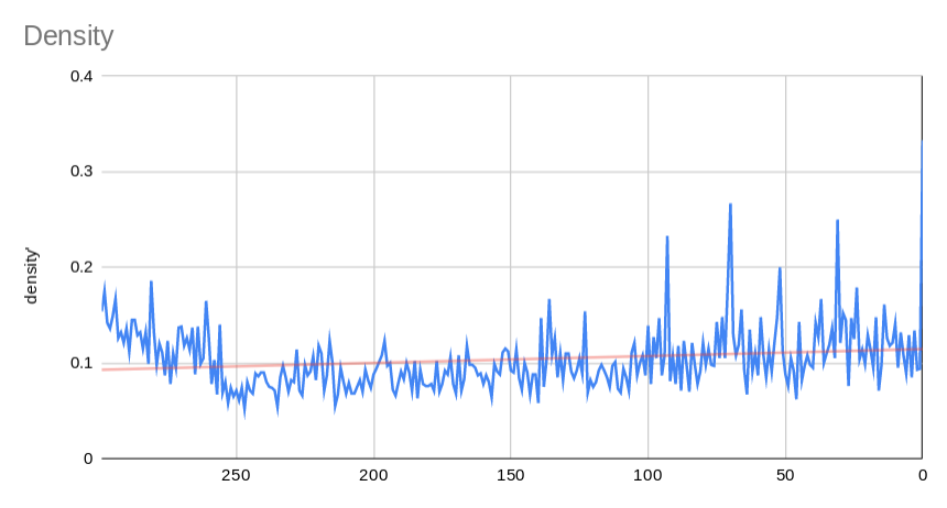
3. Third, the density of a graph is the number of existing edges over the total number of possible edges. So a graph where everyone replied to everyone would be more dense than a graph where you may have only replied to one or two other users.

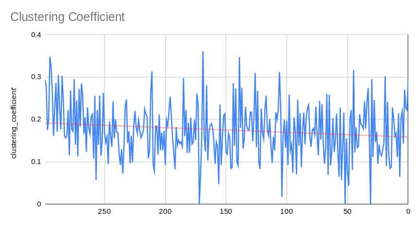
4. The clustering coefficient of a graph is the number of closed triplets over the num of total possible triplets. A closed triplet is a set of three nodes with three edges connecting them. On the other hand, an open triplet would be three nodes with 0, 1 or 2 edges connecting them.

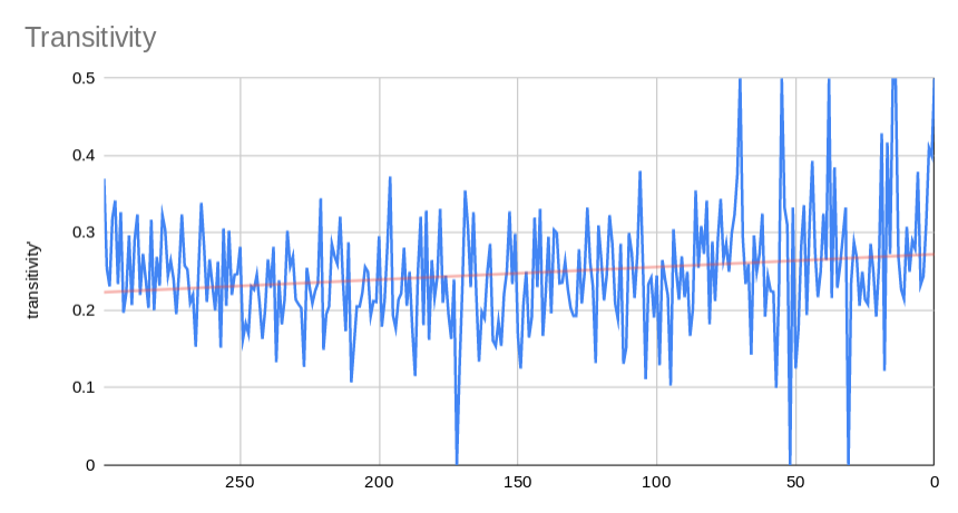
5. Transitivity is very similar to the clustering coefficient, it represents the number of triangles over the number of possible triangles. I'm not actually sure why this number is trending higher than clustering coefficent, but I think it may have to do with clustering coefficient being an average across the graph and transitivity being a global metric.

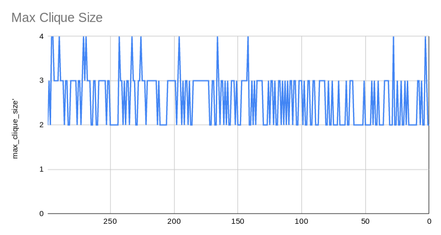
6. In network terminoloy, a max-clique is a subset of nodes where each node is connected to each other node in that subset. This graph shows the largest max-clique across all pubskis. Seems relatively stable around a max-clique size of around 2.5. Which means that on average, each Pubski has at least one group of 2 to 3 users that all reply to each other.

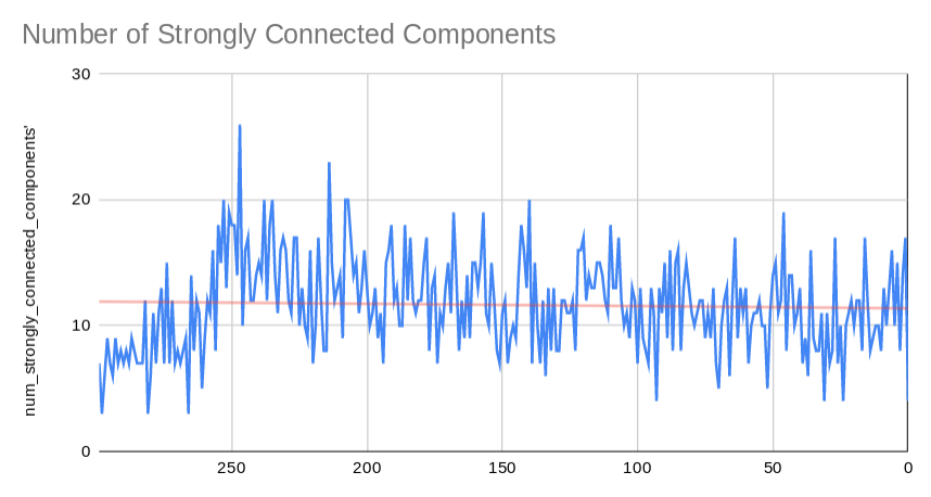
7. A strongly connected component is a subgraph where each node is connected to each other node. It is very similar to a maximal-clique, but deals with reachability rather than direct connectedness. In the case of Pubski, this metric seems to be hovering around 14. Meaning that there are on average of 14 nodes that are directly reachable from one another via a path of one or more edges.

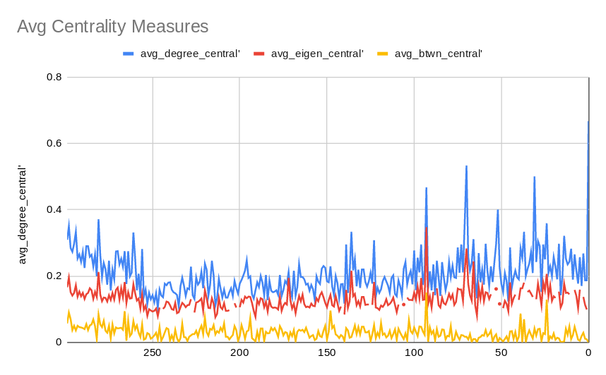
8. Centrality deals with the "importance" of a single vertex, measured by various metrics. Of course, one of the given assumptions in our specific graph is that first-level replies on a Pubski post all connect to a "Pubski Post", this should be kept in mind as we look at this metric in particular. Degree Centrality is this simplest, merely referring to the degree of a node as it's centrality score. Eigenvector Centrality has more mathematical roots, but deals with centrality as a measure of the influence of a nodes neighbors. Finally, Betweenness Centrality is a measure of how many times a given nodes falls on a shortest path.

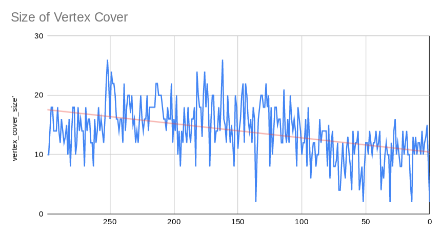
9. A vertex cover is a set of nodes with the property that each edge in the graph is incident to at least one of the nodes in the set. This metic has been in steady decline since the first pubskis. Perhaps this is related to the overall decline in number of edges we observed earlier.

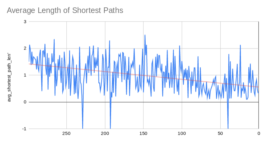
10. The shortest path between two nodes is the minimum number of edges between them. We calculate this measure for all pairs of nodes in a graph, and average them in order to get this metric. The large dips to -1 are representative of graphs where there were infinite cycles, making the calculation of shortest path impossible (they can be safely ignored).

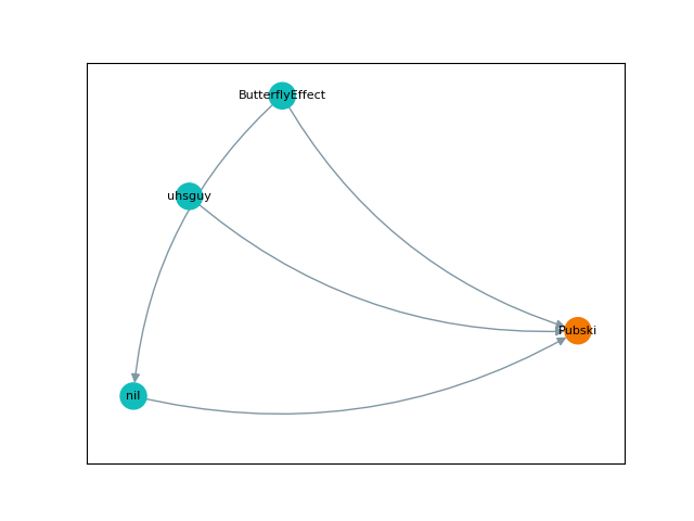
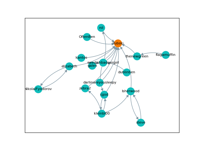
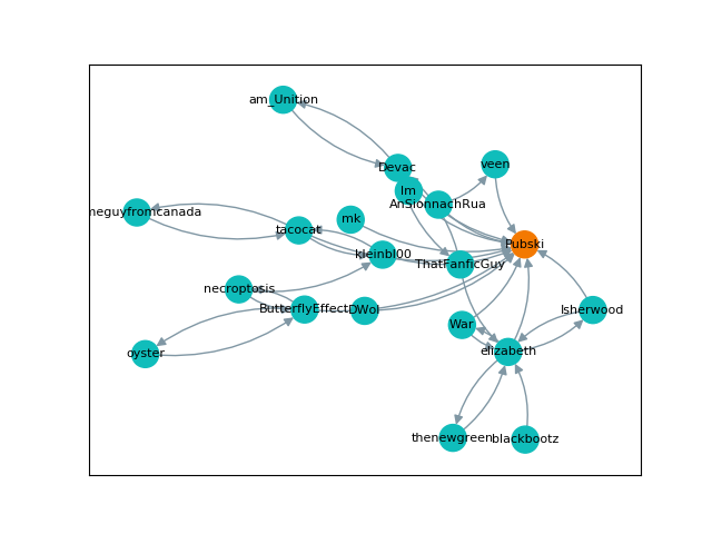
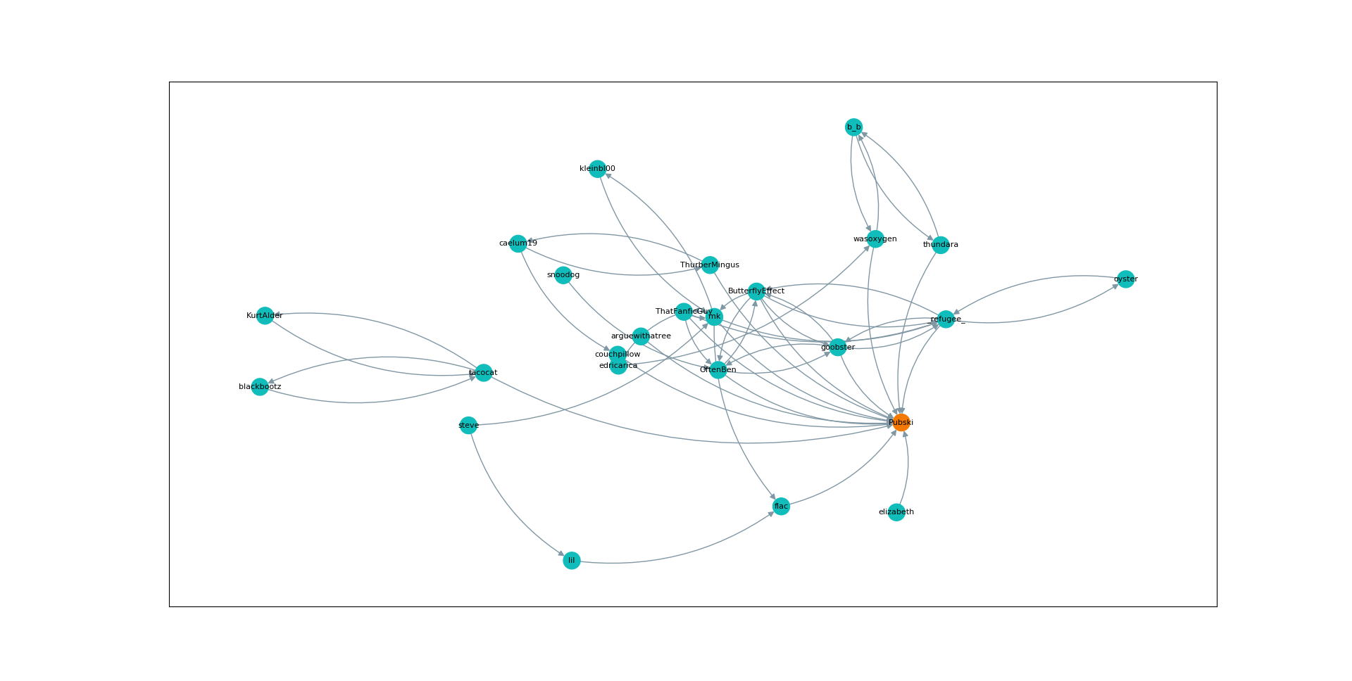
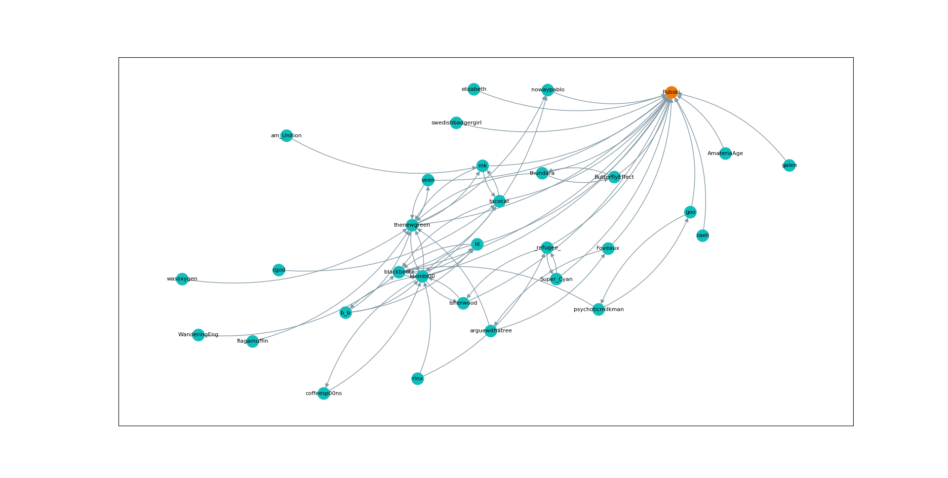
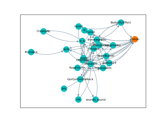
Visualization

Finally, I wanted to show off what these graphs actually looked like, so below are a few visual examples. Note that the "nil" user represents user-inactive, the Hubski term for deactivated or banned accounts. They are in chronological order, but skip around a little.